Colocalization locus plot — coloc

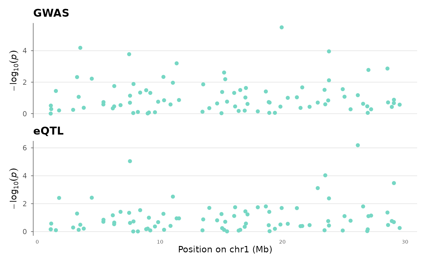
Two association signals on a shared genomic coordinate axis — the standard way to visually assess whether a GWAS signal and an eQTL (or two GWAS traits) share the same causal variant.

Usage

coloc_plot(
  gwas1,
  gwas2,
  chr = NULL,
  bp = NULL,
  p = NULL,
  snp = NULL,
  region_chr = NULL,
  region_start = NULL,
  region_end = NULL,
  lead_snp = NULL,
  flank = 5e+05,
  ld = NULL,
  ld_colors = c("#2166AC", "#67A9CF", "#78C679", "#F4A582", "#D73027"),
  top_title = "Trait 1",
  bottom_title = "Trait 2",
  highlight_snps = NULL,
  point_size = 2,
  title = NULL
)

Arguments

gwas1: First dataset (e.g., GWAS). A gwas_data or data.frame.
gwas2: Second dataset (e.g., eQTL). Same format.
chr, bp, p, snp: Column name overrides (applied to both datasets).
region_chr: Chromosome of the region to plot.
region_start, region_end: Start and end positions.
lead_snp: SNP ID to center on (± flank).
flank: Flank size in bp around lead_snp.
ld: Named numeric vector of LD r² values (optional).
ld_colors: Colors for LD bins.
top_title: Label for the top panel.
bottom_title: Label for the bottom panel.
highlight_snps: SNPs to highlight in both panels.
point_size: Point size.
title: Overall title.

Value

A patchwork composition of two locus plots.

Examples

data(example_gwas)
gwas2 <- example_gwas
gwas2$P <- runif(nrow(gwas2))^2
coloc_plot(example_gwas, gwas2,
           region_chr = 1, region_start = 1e6, region_end = 30e6,
           top_title = "GWAS", bottom_title = "eQTL")