Gene annotation track

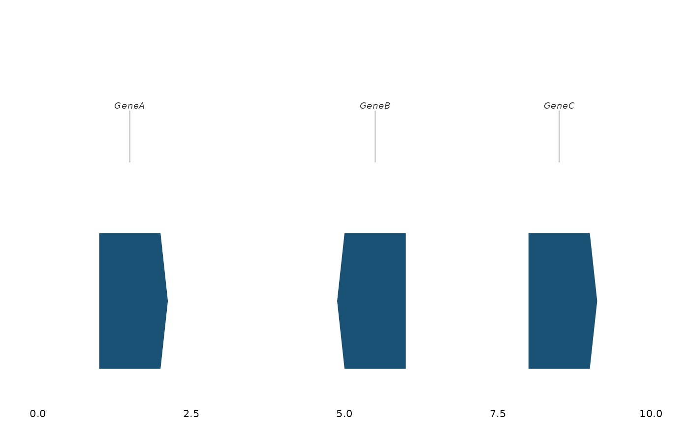
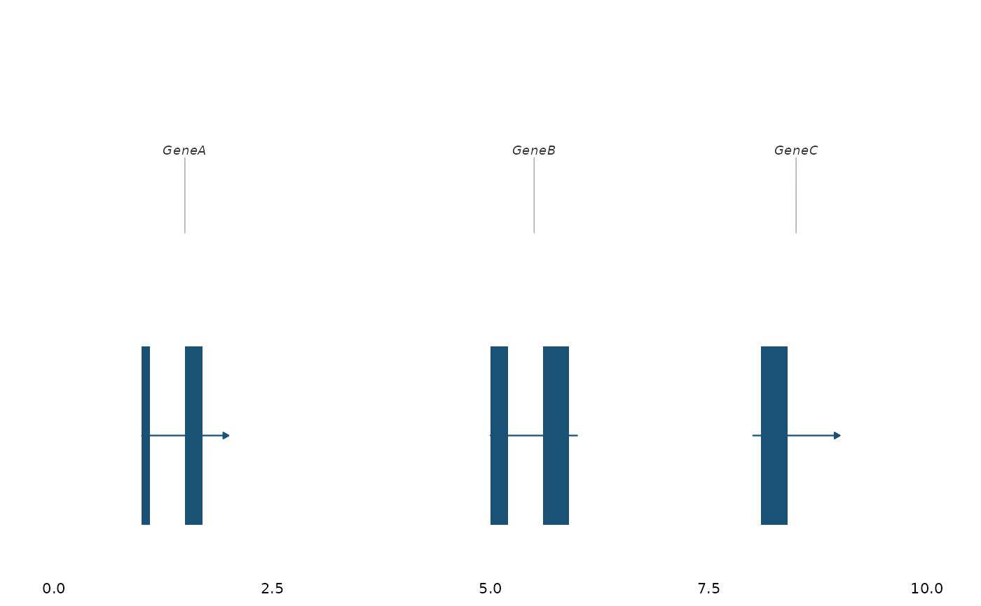
Create a standalone gene annotation panel that can be composed with any ggwas plot using patchwork. Genes are drawn as directional bodies with strand arrows and labels; when exon_data is supplied, each gene is rendered as an intron backbone with exon boxes and a strand arrow.

Usage

gene_track(
  gene_data,
  region_chr,
  region_start,
  region_end,
  exon_data = NULL,
  highlight_genes = NULL,
  highlight_color = "#E74C3C",
  label_size = 2.5,
  track_color = "#1A5276",
  show_strand = TRUE,
  max_genes = 50
)

Arguments

gene_data

A data.frame with columns: chr, start, end, gene. Optional: strand ("+"/"-").

region_chr

Chromosome to display (integer or string).

region_start, region_end

Region boundaries in base pairs.

exon_data

Optional data.frame of exons (columns chr, start, end, gene) matching genes in gene_data by the gene column. When supplied, genes are drawn with exon structure. Read with read_gtf(path, feature_type = "exon").

highlight_genes

Character vector of gene names to highlight.

highlight_color

Color for highlighted genes.

label_size

Text size for gene labels.

track_color

Default color for gene bodies.

show_strand

If TRUE, draw arrows indicating gene direction.

max_genes

Maximum number of genes to display. The longest genes are kept when the limit is exceeded.

Value

A ggplot object. Compose with a Manhattan or locus plot using patchwork::wrap_plots().

Examples

genes <- data.frame(
  chr = c(1, 1, 1), start = c(1e6, 5e6, 8e6),
  end = c(2e6, 6e6, 9e6), gene = c("GeneA", "GeneB", "GeneC"),
  strand = c("+", "-", "+")
)

# Gene-body track
gene_track(genes, region_chr = 1, region_start = 0, region_end = 10e6)


# With exon structure
exons <- data.frame(
  chr = 1,
  start = c(1.0e6, 1.5e6, 5.0e6, 5.6e6, 8.1e6),
  end   = c(1.1e6, 1.7e6, 5.2e6, 5.9e6, 8.4e6),
  gene  = c("GeneA", "GeneA", "GeneB", "GeneB", "GeneC")
)
gene_track(genes, 1, 0, 10e6, exon_data = exons)