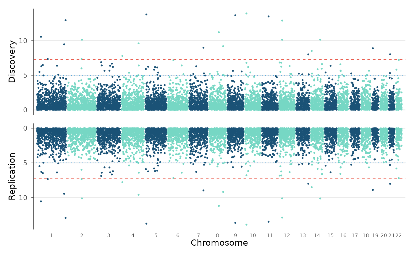
Miami plot (mirrored Manhattan) — miami

Create a Miami plot showing two GWAS results as mirrored Manhattan plots. The top panel shows one study with -log10(p) going up, and the bottom panel shows another study with -log10(p) going down.

Usage

miami_plot(
  top,
  bottom,
  chr = NULL,
  bp = NULL,
  p = NULL,
  snp = NULL,
  colors = c("#1A5276", "#76D7C4"),
  genome_wide = 5e-08,
  suggestive = 1e-05,
  top_highlight = NULL,
  bottom_highlight = NULL,
  top_label = NULL,
  bottom_label = NULL,
  top_title = NULL,
  bottom_title = NULL,
  downsample = TRUE,
  downsample_n = 2e+05,
  title = NULL
)

Arguments

top: A gwas_data object or data.frame for the top panel.
bottom: A gwas_data object or data.frame for the bottom panel.
chr, bp, p, snp: Column name overrides.
colors: Two-color vector for alternating chromosomes.
genome_wide: Genome-wide significance threshold.
suggestive: Suggestive significance threshold.
top_highlight, bottom_highlight: SNP IDs to highlight in each panel.
top_label, bottom_label: SNP IDs to label in each panel.
top_title, bottom_title: Y-axis titles for each panel.
downsample: Enable smart downsampling.
downsample_n: Target points per panel.
title: Overall plot title.

Value

A ggplot object composed via patchwork.

Examples

data(example_gwas, package = "ggwas")

# Discovery vs replication
miami_plot(example_gwas, example_gwas,
  top_title = "Discovery", bottom_title = "Replication")


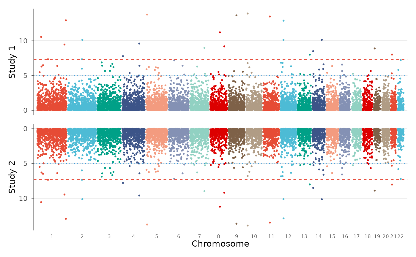
# Different colors
miami_plot(example_gwas, example_gwas,
  colors = gwas_palette("nature"),
  top_title = "Study 1", bottom_title = "Study 2")