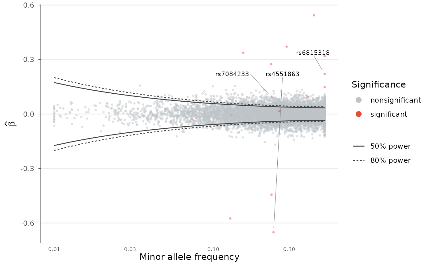
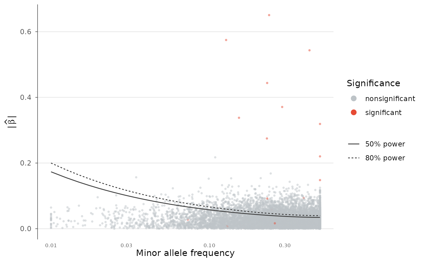
Trumpet plot: effect size versus allele frequency with power contours

Plot per-variant effect sizes against minor allele frequency and overlay statistical-power ("detection") contours. The contours trace the smallest effect a study of the given sample size can detect at a chosen significance level and power, producing the characteristic trumpet shape that flares toward rare variants. Points falling below all contours lie in the region a study is underpowered to discover.

Usage

trumpet_plot(
  data,
  beta = NULL,
  af = NULL,
  p = NULL,
  n = NULL,
  n_col = NULL,
  sig_level = 5e-08,
  power = c(0.5, 0.8),
  signed = FALSE,
  colors = c(significant = "#E64B35", nonsignificant = "#BDC3C7"),
  point_size = 1,
  alpha = 0.5,
  label_top_n = NULL,
  title = NULL
)

Arguments

data: A gwas_data object or data.frame with BETA and AF columns.
beta, af, p: Column name overrides.
n: Study sample size (single number). If NULL, taken from n_col or an N column (median).
n_col: Name of a per-variant sample-size column.
sig_level: Significance threshold for the power contours.
power: Numeric vector of power levels to draw contours for.
signed: If TRUE, plot signed effects (contours mirrored above and below zero); otherwise plot the absolute effect.
colors: Named vector with "significant" and "nonsignificant" colors.
point_size: Point size.
alpha: Point transparency.
label_top_n: Label the top N variants by significance.
title: Plot title.

Value

A ggplot object.

Details

The power model assumes an additive test on a standardized quantitative trait (per-allele effect on a unit-variance scale). For each minor allele frequency \(f\), the minimum detectable effect is \(\beta_{min}(f) = \sqrt{\lambda / (2 N f (1 - f))}\), where the non-centrality parameter \(\lambda = (z_{\alpha} + z_{power})^2\).

Examples

data(example_gwas)

# Effect size versus MAF with 50% and 80% power contours
trumpet_plot(example_gwas, n = 50000)


# Signed effects and a labelled top hit
trumpet_plot(example_gwas, n = 50000, signed = TRUE,
             p = "P", label_top_n = 3)